Toggle navigation

.ipynb .pdf

repository open issue

Contents

Online Analysis

Being able to visualize and interpret simulation data in real time is invaluable for understanding the behavior of a physical system.

SmartSim can be used to stream data from Fortran, C, and C++ simulations to Python where visualization is significantly easier and more interactive.

This example shows how to use SmartSim analyze the vorticity field during a simple, Python based Lattice Boltzmann fluid flow simulation.

Lattice Boltzmann Simulation

This example was adapted from Philip Mocz’s implementation of the lattice Boltzmann method in Python. Since that example is licensed under GPL, so is this example.

Philip also wrote a great medium article explaining the simulation in detail.

Integrating SmartRedis

Typically HPC simulations are written in C, C++, Fortran or other high performance languages. Embedding the SmartRedis client usually involves compiling in the SmartRedis library into the simulation.

Because this simulation is written in Python, we can use the SmartRedis Python client to stream data to the database. To make the visualization easier, we use the SmartRedis Dataset object to hold two 2D NumPy arrays. A convenience function is provided to convert the fields into a dataset object.

# Select lines from updated simulation code highlighting
# the use of SmartRedis to stream data to another processes

from smartredis import Client, Dataset
client = Client() # Addresses passed to job through SmartSim launch

# send cylinder location only once
client.put_tensor("cylinder", cylinder.astype(np.int8))

for i in range(time_steps):
    # send every 5 time_step to reduce memory consumption
    if time_step % 5 == 0:
        dataset = create_dataset(time_step, ux, uy)
        client.put_dataset(dataset)

def create_dataset(time_step, ux, uy):
    """Create SmartRedis Dataset containing multiple NumPy arrays
    to be stored at a single key within the database"""
    dataset = Dataset(f"data_{time_step}")
    dataset.add_tensor("ux", ux)
    dataset.add_tensor("uy", uy)
    return dataset

This is all the SmartRedis code needed to stream the simulation data. Note that the client does not need to have an address explicitly stated because we are going to be launching the simulation through SmartSim as shown in the cell below

import time
import numpy as np
import matplotlib.pyplot as plt

from smartredis import Client
from smartsim import Experiment
from vishelpers import plot_lattice_vorticity

Starting the Experiment

SmartSim, the infrastructure library, is used here to launch both the database and the simulation locally, but in separate processes. The example is designed to run on laptops, so the local launcher is used.

First the necessary libraries are imported and an Experiment instance is created. An Orchestrator database reference is intialized and launched to stage data between the simulation and this notebook where we will be performing the analysis.

# Initialize an Experiment with the local launcher
# This will be the name of the output directory that holds
# the output from our simulation and SmartSim
exp = Experiment("finite_volume_simulation", launcher="local")

# create an Orchestrator database reference,
# generate it's output directory, and launch it locally
db = exp.create_database(port=6780, interface="lo")
exp.generate(db, overwrite=True)
exp.start(db)
print(f"Database started at address: {db.get_address()}")

Database started at address: ['127.0.0.1:6780']

Running the Simulation

To run the simulation, Experiment.create_run_settings is used to define how the simulation should be executed. These settings are then passed to create a reference to the simulation through a call to Experiment.create_model() which can be used to start, monitor, and stop the simulation from this notebook.

Once the model is defined it is started by passing the reference to Experiment.start() The simulation is started with the block=False argument. This runs the simulation in a nonblocking manner so that the data being streamed from the simulation can be analyzed in real time.

# set simulation parameters we can pass as executable arguments
time_steps, seed = 3000, 42

# create "run settings" for the simulation which define how
# the simulation will be executed when passed to Experiment.start()
settings = exp.create_run_settings("python",
                                   exe_args=["fv_sim.py",
                                             f"--seed={seed}",
                                             f"--steps={time_steps}"])

# Create the Model reference to our simulation and
# attach needed files to be copied, configured, or symlinked into
# the Model directory at runtime.
model = exp.create_model("fv_simulation", settings)
model.attach_generator_files(to_copy="fv_sim.py")
exp.generate(model, overwrite=True)

22:50:07 e3fbeabfdb3e SmartSim[1216] INFO Working in previously created experiment

# start simulation without blocking so data can be analyzed in real time
exp.start(model, block=False, summary=True)

22:50:07 e3fbeabfdb3e SmartSim[1216] INFO

=== Launch Summary ===
Experiment: finite_volume_simulation
Experiment Path: /home/craylabs/tutorials/online_analysis/lattice/finite_volume_simulation
Launcher: local
Models: 1
Database Status: active

=== Models ===
fv_simulation
Executable: /usr/bin/python
Executable Arguments: fv_sim.py --seed=42 --steps=3000

Online Visualization

SmartRedis is used to pull the Datasets stored in the Orchestrator database by the simulation and use matplotlib to plot the results.

In this example, we are running the visualization in an interactive manner. If instead we wanted to encapsulate this workflow to deploy on an HPC platform we could have created another Model to plot the results and launched in a similar manner to the simulation. Doing so would enable the analysis application to be executed on different resources such as GPU enabled nodes, or distributed across many nodes.

# connect a SmartRedis client to retrieve data while the
# simulation is producing it and storing it within the
# orchestrator database
client = Client(address=db.get_address()[0], cluster=False)

# Get the cylinder location in the mesh
client.poll_key(f"cylinder", 300, 1000)
cylinder = client.get_tensor("cylinder").astype(bool)

# plot every 700th timestep
for i in range(0, time_steps + 1, 700):
    client.poll_dataset(f"data_{i}", 300, 1000)
    dataset = client.get_dataset(f"data_{i}")
    ux, uy = dataset.get_tensor("ux"), dataset.get_tensor("uy")

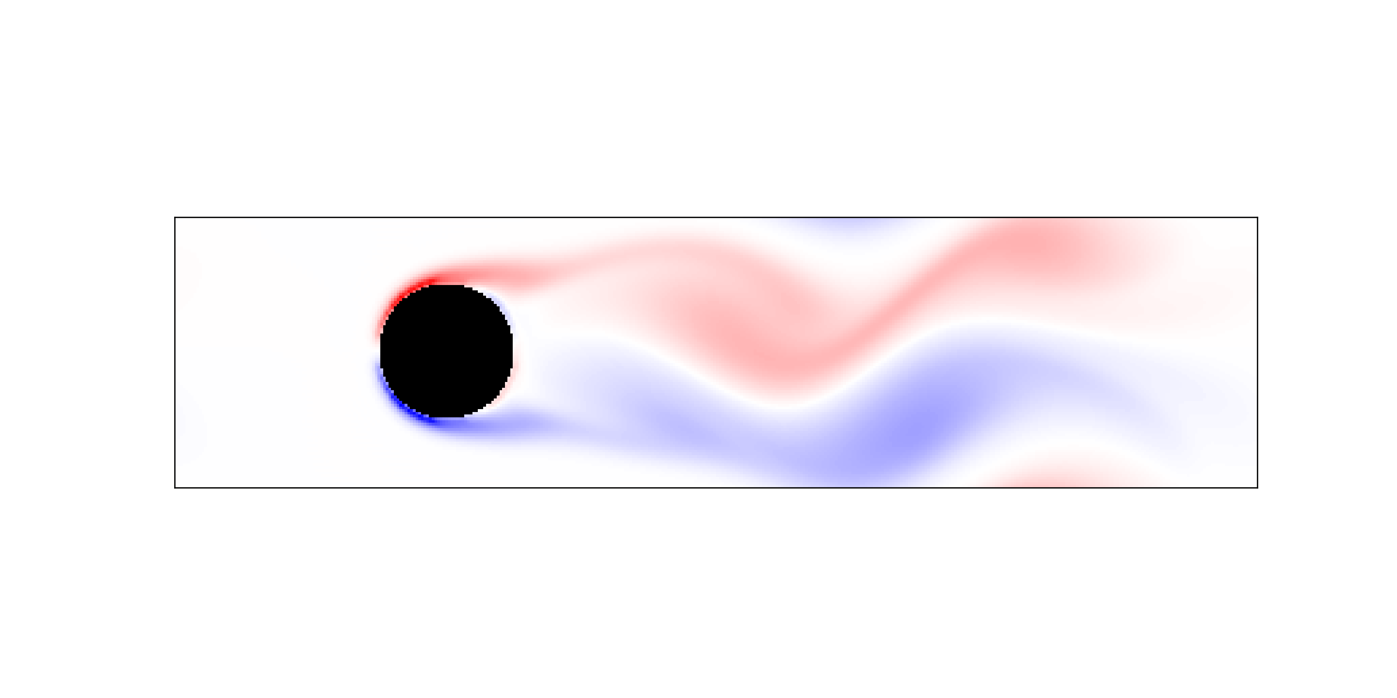
    plot_lattice_vorticity(i, ux, uy, cylinder)

Vorticity plot at timestep: 0

Vorticity plot at timestep: 700

Vorticity plot at timestep: 1400

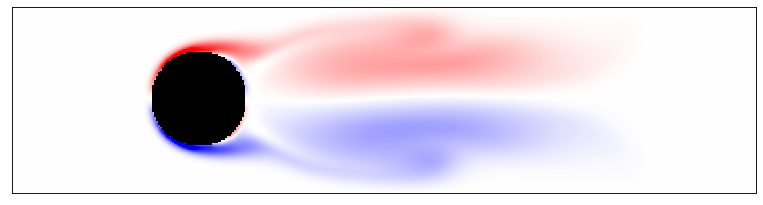
Vorticity plot at timestep: 2100

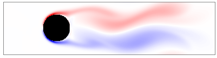
Vorticity plot at timestep: 2800

# Optionally clear the database
client.flush_db(db.get_address())

# Use the Experiment API to wait until the model
# is finished and then terminate the database and
# release it's resources
while not exp.finished(model):
    time.sleep(5)

exp.stop(db)

22:50:59 e3fbeabfdb3e SmartSim[1216] INFO fv_simulation(1337): Completed
22:51:01 e3fbeabfdb3e SmartSim[1216] INFO Stopping model orchestrator_0 with job name orchestrator_0-CI23BKDK76I0
22:51:11 e3fbeabfdb3e SmartSim[1216] WARNING Unable to kill emitted process 1327

exp.get_status(model)

['Completed']

exp.summary(format="html")

	Name	Entity-Type	JobID	RunID	Time	Status	Returncode
0	fv_simulation	Model	1337	0	41.7211	Completed	0
1	orchestrator_0	DBNode	1322	0	83.3787	Cancelled	-9

previous

Getting Started

next

Online Inference